Primes' Gaps & Zeros of the Completed Riemann ζ Function
Technical Introduction
This construction is an observational tool for placing two established mathematical datasets in one measured circular field: consecutive gaps between primes and consecutive gaps between positive ordinates of nontrivial zeros of the Riemann zeta function represented on the critical line.
The map terminates at 1009 Map Units. The same interval, the same North cut, the same clockwise direction, and the same angular translator are used for both datasets. The construction therefore permits the position of every cut and the measure of every gap to be recovered analytically in a common unit.
The drawing is a scheme of the instrument. It is not itself a measuring surface, and no mathematical conclusion should be obtained by applying a compass or ruler to the screen. The drawing identifies coordinates, cuts, sectors, and possible observations. All measurements must be returned to the stored numerical data and calculated analytically.
Concise Legend
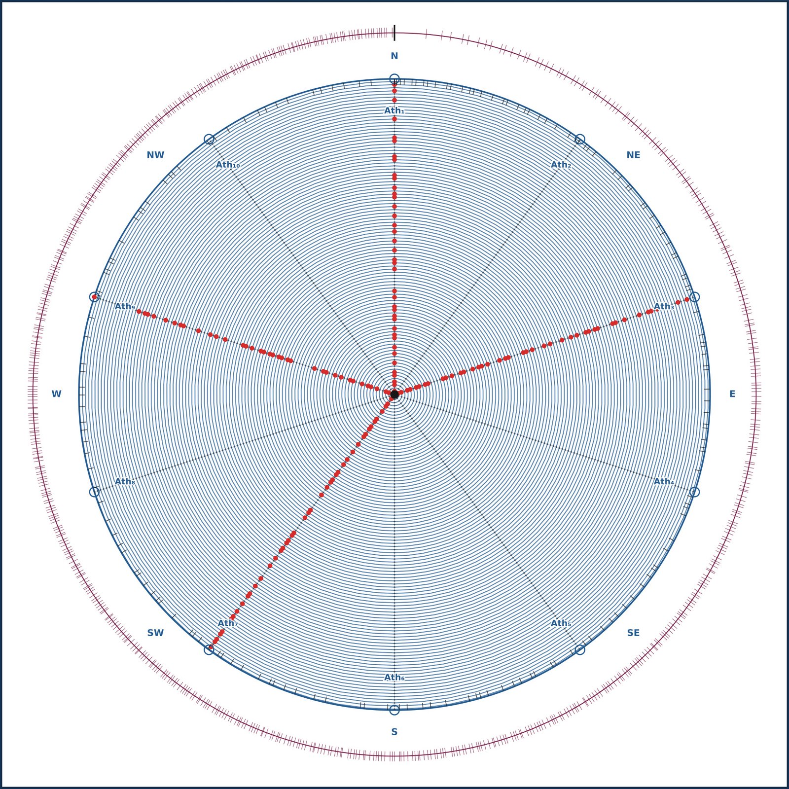
Blue spiral: Archimedean spiral encoding the ordered mathematical line up to 1009.
Red points: primes placed at their Map Unit coordinates on the spiral.
Ath₁–Ath₁₀: ten circular atoms, numbered clockwise from North.
Rose of the Winds: independent directional reference
Prime-gap horizon: sectors determined by consecutive prime cuts.
Outer red-violet ring: cuts determined by positive nontrivial zeta-zero ordinates 0 < γ ≤ 1009.
North cut: beginning and end of the circularized measured line; γ = 0 is a reading origin, not a zeta zero.
Scientific Layer
Classical Mathematics supplies the primes pₙ, the consecutive prime gaps, the nontrivial zeta-zero ordinates γₘ represented here, and the consecutive differences between those ordinates. It also determines the mathematical status of every datum used by the instrument.
Circular Mathematics supplies the observational map: circularization of a finite measured line, a cut preserving its beginning and end, a common direction of reading, layered rings, and reversible translation between Map Units and circular angle. Circularization does not change the classical data and does not by itself establish a correlation between the two distributions.
In the present dataset there are 169 primes and 168 consecutive prime gaps from 2 through 1009. The outer ring contains 656 positive zeta-zero ordinates and therefore 655 consecutive zero gaps. Negative ordinates are not separately drawn in this layer.
The Spiral as a Measured Line
The Archimedean spiral represents an ordered mathematical line through its numerical parameter. A prime pₙ is placed at the coordinate pₙ. When the spiral is conceptually unrolled, the classical prime position is recovered without alteration.
pₙ → pₙ[1]
A prime gap is not the visible straight distance between two consecutive primes
(represented in the drawing as “stars”), nor is it the curved arc length of the
spiral. It is the difference between their numerical coordinates:
Gₚ = (pₙ₊₁ − pₙ)[1]
The spiral is therefore a visual encoding of the line; the Map Unit coordinate remains the source of measurement.
Map Unit
The basic unit is one Map Unit, written [1]. It is one coordinate unit of the mathematical map, comparable to one unit on an x-y grid. It is not a meter or another physical unit.
[1] = one Map Unit
Prime positions and prime gaps are integer multiples of [1]:
pₙ[1]
Gₚ = (pₙ₊₁ − pₙ)[1]
The positive zeta-zero ordinate γₘ is assigned a position on the same mathematical map. Its coordinate and the difference between consecutive ordinates use the same unit:
γₘ[1]
Gζ = (γₘ₊₁ − γₘ)[1]
Prime gaps are integer multiples of [1]. Zeta-zero gaps are generally fractional multiples of [1]. Assigning the same Map Unit does not identify primes with zeta zeros; it gives their positions and gaps a common coordinate scale for observation.
Simple Circular Translation
The measured line begins at 0[1] and ends at 1009[1]. Circularization maps that complete interval onto one turn while preserving the North cut as its beginning and end.
2π radians = 360° = 400 gon = 100%
For any position x[1] on the measured line:
θ(x) = 2πx / 1009
Percent(x) = 100x / 1009 %
Degrees(x) = 360x / 1009 °
Gradians(x) = 400x / 1009 gon
One Map Unit therefore receives the exact translations:
[1] → 2π / 1009 radians
[1] → 100 / 1009 %
A gap G[1], whether a prime gap or a zeta-zero gap, becomes:
G[1] → 2πG / 1009 radians
G[1] → 100G / 1009 %
The translation is reversible. Every angular observation can be returned to the measured mathematical line:
x[1] = 1009θ / 2π [1]
x[1] = 1009 × Percent(x) / 100 [1]
Placement and Separation
A prime cut pₙ and a zeta-zero cut γₘ can be checked on the same circularized line. Their separation is first calculated in Map Units:
Δ[1] = |pₙ − γₘ|[1]
It can then be expressed as circular angle or percentage:
Δθ = 2π|pₙ − γₘ| / 1009
ΔPercent = 100|pₙ − γₘ| / 1009 %
Because the circularized line retains a beginning and an end, the instrument uses the ordinary distance on the source line. It does not replace that distance with the shortest route around an uncut circle.
Precision and Computational Margin
The Map Unit translation is exact. Prime positions and prime gaps are exact integer data. The numerical margin enters through the decimal representation of the zeta-zero ordinates used by the computer.
The ordinates in the current dataset are recorded to nine places after the decimal point. Rounding to nine decimal places gives a maximum margin of one-half of the final retained decimal unit:
eγ ≤ ½ × 10⁻⁹[1] = 5 × 10⁻¹⁰[1]
This is one-half of one billionth of a Map Unit. For a gap calculated from two independently rounded ordinates, the conservative maximum margin is:
eGζ ≤ 10⁻⁹[1]
The corresponding angular and percentage margins for one zero cut are:
eθ ≤ 2π(5 × 10⁻¹⁰) / 1009
eθ ≈ 3.11 × 10⁻¹² radians
e% ≤ 100(5 × 10⁻¹⁰) / 1009 %
e% ≈ 4.96 × 10⁻¹¹ %
This is a numerical-computation margin, not an error inherent in the exact mathematical construction. It is relevant to analytic calculation but marginal at the present scale.
Map Unit and Interface Pixel
For translation into the computer observation interface, one Map Unit corresponds theoretically to one interface pixel:
[1] ↔ 1 interface pixel
The interface pixel is independent of the dimensions of the exported drawing, browser scaling, screen resolution, and human eyesight. It belongs to the underlying computer map rather than to a particular JPEG.
Under this correspondence, the nine-decimal margin becomes:
5 × 10⁻¹⁰[1] ↔ 5 × 10⁻¹⁰ interface pixel
A zeta ordinate may therefore occupy a fractional interface-pixel coordinate. The computer eye reads the stored coordinate, while the visible drawing presents a schematic projection for human navigation.
Drawing and Analytic Measurement
The drawing is only a drawing: a schematic visualization of the instrument. It is not used for direct screen measurement. Visible distance, angle, line thickness, and apparent overlap are not substitutes for calculation.
The drawing supplies a tool for locating an observation. Once a cut, sector, gap, or apparent alignment has been selected, the interface retrieves its stored Map Unit coordinates and performs the measurement analytically.
numerical data → schematic drawing → selected observation → analytic measurement
The computer eye reads coordinates. The human eye navigates the scheme.
Scientific Status and Potential Use
The construction is presently a visualization, encoding, and observational tool. It can be used for mathematical education, verification of data placement, exploratory observation, selection of candidate alignments, and the design of analytic tests.
It does not yet establish a pattern, prediction, correlation, or theorem connecting prime gaps with zeta-zero gaps. The unequal numbers of gaps prevent an automatic one-to-one pairing. Any statistical investigation must separately declare its comparison rule, normalization if required, and test against chance.
The present function is more elementary and more exact: it places both datasets on one measured line, translates them into one circular field, and allows every selected visual observation to be recovered analytically.
Fraction of Infinity — Circular Mathematics Note

Fraction of Infinity
Fraction of Infinity
is introduced in the Crystal Basic section. It describes a fraction whose
denominator extends toward infinity while the fraction approaches zero
without being treated as zero at the selected resolution.
1/n → 0 as n → ∞
In Circular Mathematics, the general Fraction of Infinity is represented
by the rune {&ww&}. A lower index identifies its observational
level within a developing hierarchy.
1
{&ww&}α
The present computational margin,
5 × 10⁻¹⁰[1], is nonzero in calculation but negligible relative to one
interface pixel. It is therefore recorded as a particular example of
Fraction of Infinity α: the first threshold beneath the
directly visible resolution of the current observation.
5 × 10⁻¹⁰[1]
↔
5 × 10⁻¹⁰ interface pixel
→
1/{&ww&}α
The notation does not replace the calculated error bound. It classifies
that bound within Circular Mathematics after the technical calculation has
been completed.
Provisional hierarchy
α — observational edge:
a nonzero fraction lying beneath the selected visibility or interface
resolution. The present nine-decimal computational margin is the first
recorded example.
β — reserved level:
a finer analytic or technological threshold whose definition has not yet
been established. No value is assigned here.
γ — proposed physical-scale level:
a possible future class for fractions approaching the scale at which the
current physical description reaches its natural boundary. The Planck
scale may be investigated as a candidate, but it is not translated
directly from the Map Unit or interface pixel in the present construction.
δ — emergence:
the boundary at which the established map no longer supplies a sufficient
description and a new physical or mathematical structure may be required.
This level remains open.
1/{&ww&}α
→
1/{&ww&}β
→
1/{&ww&}γ
→
δ
The hierarchy is directional rather than numerical at this stage. It
organizes examples by their relation to observation, resolution,
technological reach, and the boundary of the established map.
In classical terms, 5 × 10⁻¹⁰[1] remains a finite numerical bound, not a
classical infinitesimal. “Fraction of Infinity” is the Circular Mathematics
interpretation of that bound within a selected observational resolution.
The scientific calculation and its Circular Mathematics classification
remain explicitly separated.
MAGE NAVIGATION INSTRUMENT
From Observation to Navigation
The scientific construction enters the MAGE navigation console as a computer-based observational instrument visualized for the human eye. The scientific layer remains independent: it defines the data, units, translations, precision, and limits of measurement. MAGE applies that completed layer as a navigational interface.
The drawing allows a human navigator to select regions, cuts, sectors, and apparent alignments. The computer eye then returns to the underlying Map Unit coordinates, reads the stored prime and zeta-zero data, and performs the requested comparison analytically.
Map Unit → circular position → interface pixel → analytic return
In this role, the circle is not decorative and the screen is not a ruler. The circle organizes navigation through the data; the numerical map remains the measuring instrument.
//to edit//
Model of Time-Space
A possible application of the model is presented separately on the
Research page.
Coding rules are being conceived in
Crystal Basic page.
Calendars
Clocks
The first temporal construction is Circular Time.
A selected recurring process is represented as a closed cycle with
finite resolution.
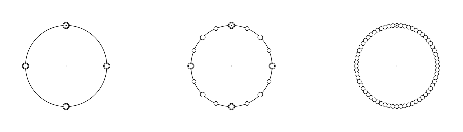
The drawing presents three levels of resolution within one cycle.
Four Phases establish its principal divisions.
Eight Gongs organize sixteen moments.
64 instants complete the selected temporal resolution.
Each resolution defines a level of measurement and observation within
the same cycle. An instant records a position at the selected
resolution. When an observed event is assigned to that position, the
instant may acquire the status of a moment, a
Border-Moment, or another defined
Timing.
Circular Mathematics
The Model of Time-Space is based on
Circular Mathematics.
Its foundational object is the Transcendental Node,
introduced in Crystal Basic as:
[−∞ 0 +∞]
Transcendental Node is constructed by identifying the two unbounded
directions and numerical zero on the extended real line:
−∞ ∼ 0 ∼ +∞
𝔗 = ℝ̄ / ∼
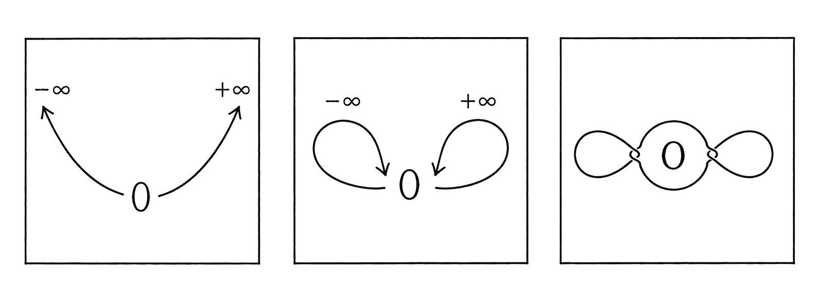 Knotting the Transcendental Node
This identifying operation is called knotting. It produces
one distinguished structural Origin ⊙ and two
complementary loops sharing that Origin:
𝔗 = 𝐿⁻ ∨⊙ 𝐿⁺
The complete two-loop structure 𝔗 is Transcendental Node.
Circular Time uses one loop as its working circular map, while the
complementary loop retains the corresponding reflected construction.
Recursive subdivision gives this map a selected finite resolution
N. Its terminal resolved elements are
Athoms, represented by Athomic Dots together with their
associated cells. [Ma] records the recursive possibility
remaining before completion. At the selected terminal resolution:
[Ma]ₙ = 0
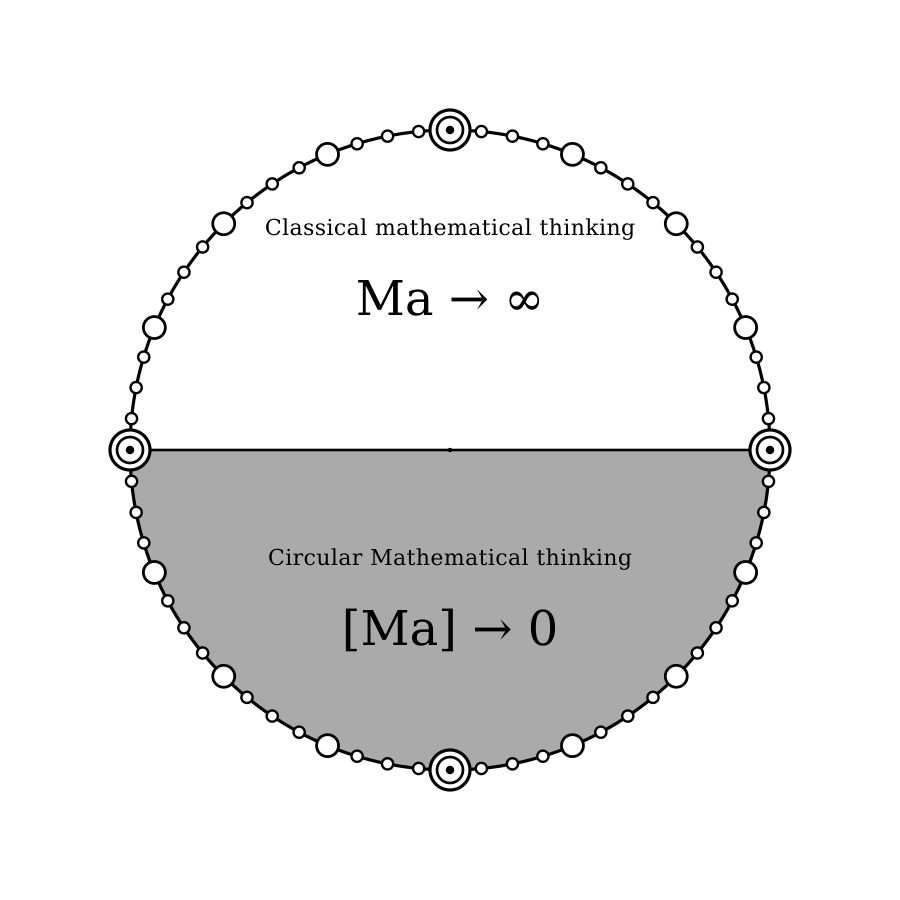
The complete construction of Transcendental Node, Origin, the Circular
Realm, Athoms, and [Ma] is presented in
Circular Mathematics.
Axioms of Circular Time
(*) The Circle with No Operative Zero or Infinity
The circle is the basic computational space of Circular Time.
Circular Time does not use zero or infinity as operative numerical
values in its computations.
Every construction begins with finite distinction and proceeds
through a selected finite resolution.
The structural Origin ⊙ is the invariant position
of joining, departure, return, and possible renewal.
There is only one Origin ⊙ per circle / ring / cycle.
[Ma] represents the required recursive possibility
that remains unresolved relative to the selected terminal
resolution. In [Ma]ₙ =" 0", zero declares the
completed status of the defined construction.
[Ring of Athoms] = "1" - the cycle is completed.
The symbols −∞ and +∞ may identify
unbounded directions brought into structural relation with the
Origin. Infinity does not enter the computation as a numerical
value.
(**) Determined Rotation
The circular structure has no arbitrarily pre-assigned direction.
Before a computation or observation begins, its rotation is
determined from the conditions of the operation and its frame of
reference.
6 — clockwise rotation
9 — counterclockwise rotation
Once determined, the rotational direction remains fixed for that
operation unless an explicit transformation changes or reverses it.
Rotation supplies the directional arrow of Circular Time.
(***) Closure and Temporal Extent
Every defined cycle of Circular Time operates at a selected finite
resolution and closes by returning to its structural Origin.
The temporal positions of the cycle are represented by Dots with
thickness. Their thickness gives them positive represented extent
and may carry information about temporal duration, intensity, or
significance.
The structural Origin remains thicknessless, even when a terminal
Dot occupies the same represented position at the completion of
the cycle.
(****) Timing and the Mapping of Events
The structure of Circular Time serves as a map upon which observed
events may be placed and compared.
An instant records a position at the selected
resolution. A moment is a position defined by an
observed event or action. A Border-Moment marks a
significant transition, boundary, or change.
A Timing is the operational unit created when an
observed event is placed upon the structure of Circular Time.
Crystal Timings
The first working alphabet of Timings uses the two determined
rotations, 6 and 9, across six positions. Its structural reference is
the binary construction of the I Ching.
{6, 9}6 = 64
The resulting 64 Crystal Timings are developed as complete Sets in
Crystal Basic.
Axiom of the Gate
(*****) Conditional Gate
The completion of a temporal cycle permits the possible generation
of a Gate.
Closure is necessary for the Gate. The Gate is generated when the
additional conditions defined for the operation have been
satisfied.
When generated, the Gate may permit passage to another level of
computation, another level of observation, another cycle or
resolution, or another level of organization within the model.
Space
The second construction of the model begins with four elementary
spatial signs:
α · β · γ · δ
Their structure takes inspiration from the genetic alphabet. Four
elementary signs arranged across three ordered positions produce
64 possible spatial configurations.
{α, β, γ, δ}3 = 64
The signs α, β, γ, and δ
The complete spatial alphabet is developed as a Set in
Crystal Basic.
Crystal Basic.